Supervised Machine Learning
Explainable Models for Geologists
Supervised learning models are those where labelled datasets are used to train a machine learning model.
There are two main types of supervised machine learning models.
- Classification models which allow the geologist to predict a category such as a rocktype (e.g. basalt, andesite, rhyolite), alteration style, weathered vs freshrock, etc.
- Regression models which predict a continuous variable such as rock properties (e.g. hardness), Au concentration using spectral data, etc.
When built by exploration teams these models can be very powerful. They amplify existing geological work and help geologists test new or existing hypotheses – such as which elements drive logged rock type predictions, or which elements and minerals influence grindability.
There are many applications where classification models can guide the exploration process, such as training a classifier on logging data from diamond drill core and using this model to predict rock types in RC drilling or legacy drillhole data where access to the samples is impossible.
One of the valid criticisms of machine learning has been the black box nature of model output. Recent advances in machine learning has now led to the development of “explainable machine learning models”, which provide per sample explainability (i.e. provide the geologist with information as to why the algorithm made the prediction that it made). Models are not perfect and arming exploration teams with prediction explainability allows the geologist to more thoroughly question model outputs (please see example below).
“All models are wrong, but some are useful.”
Value
- Leverage existing geological models to predict new or previously unlogged samples.
- Explainable ML reveals why each prediction was made allowing geologists to critically evaluate outputs rather than accepting them blindly.
- Quantify and reduce risk using recent advances in uncertainty modelling (e.g. conformal prediction), so every prediction has a confidence measure – not a probability score.
Rocktype classification example
Below is a map of sedimentary rock samples from the South Island of New Zealand. These rocks belong to either the more recent Caples Group, or older Sedimentary units such as the Torlesse Group. These two sedimentary packages (i.e. Caples Sediments vs Other Sediments) have been confirmed in previous studies using multi-element geochemistry as well as isotopic analysis.
For gold exploration it is important to know whether you are outside or inside the Caples Group. Other Sediments outside the Caples Group have higher prospectivity for gold mineralisation. Although some gold deposits can be seen in the South Eastern portion of the Caples Group, this portion of the Caples is quite thin and not representative of the rest of the Caples. The central and western portions of the Caples Group are much thicker and do not host gold mineralisation. Unfortunately for geologists, sedimentary units from outside the Caples look almost identical to those from within the Caples Group. Isotopic analysis is able to separate these two packages of rock fairly easily, however this method is expensive with a long lead time for results.
For this reason geologists were interested in training a supervised model using geochemical samples from both packages so future samples could be classified using only wholerock geochemical values without the need for isotopic analysis saving both money and time.
Below is a map showing the 94 samples which were used to train the model as well as the three samples which required classification. The labels for these samples were confirmed as being “Caples Group” or “Other Sediments” using isotopic analysis, but importantly only whole rock geochemical data was used to train the model.
The CatBoost machine learning model was trained and evaluated using k-folds cross validation (with 5 folds). The training data was partitioned into 5 datasets — the model trains on 4 of them, evaluates on the remaining one, and repeats until each partition has been used as the evaluation set. The tuned model was then applied to a separate test set that played no role in training or tuning.
The results above show that the model correctly classified 86 of the 94 training samples under cross-validation, with 4 known Caples samples misclassified as Other Sediments and 4 samples known to be Other Sediments misclassified as Caples Group. On the independent test set of 24 completely unseen samples, the model correctly classified 23 – misclassifying just one Caples Group sample – and identified every Other Sediments sample correctly. The test performance exceeding cross-validation is a strong indicator that the model generalises well and is not overfitted to the training data.
Explainable ML – SHAP Values
The great thing about tree-based supervised models is they allow for the computation of explainable ML outputs. These do not just inform the user of what is important for the overall model, but they inform the user why the model made each individual prediction.
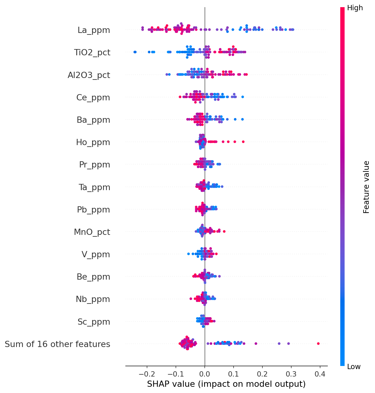
SHAP (SHapley Additive exPlanations) values quantify the contribution of each geochemical variable to every individual prediction. Rather than treating the model as a black box, SHAP decomposes each prediction so we can see if a given geochemical assay value pushed or pulled the model toward one group or the other. The beeswarm plot below summarises SHAP values across the entire training set. Each point is a sample, its position on the x-axis is its SHAP value with higher values pushing the model towards a prediction towards the Caples Group, and lower values pulling the prediction towards the Other Sediment group. The colour of the point represents the value for that geochemical variable (i.e. red points relatively high concentrations with relatively low concentrations coloured blue).
Here we can see that La values are the most important in discriminating between these two groups with lower La values pushing the prediction towards the Caples Group and higher values pulling the prediction towards the Other Group. To the right of the beeswarm plots we have waterfall plots which provide explainability for the three unlabelled sediment samples. The SHAP value is coloured by whether the assay value for that specific sample pushed the prediction towards a Caples Group prediction (blue bar) or pulled towards an Other Sediment prediction (orange bar).
Sample P64032 was predicted as belonging to the Caples Group and the waterfall plot shows that all variables listed in the plot had SHAP values which pushed towards that prediction. Sample P64029 was predicted as belonging to the Other Sediments group, with Pb being the only variable here that pushed the prediction towards the Caples Group. While Sample OU63218 had a somewhat more mixed signature with many variables such as La and Ce pulling the prediction towards the Other Sediments group, while elements such as Yb and Tm pushed towards the Caples Group.
These explainability plots allowed the geologist to question the predictions made for specific samples.
Measuring uncertainty – conformal prediction
Supervised classification algorithms always provide a probability value that a sample belongs to each possible class. These values range between 0 and 1 and the predicted label is the one with the highest probability value.
These probability values are useful but are uncalibrated. By uncalibrated I mean that a probability of > 0.7 may be conclusive for one model, but may be ambiguous for another machine learning model.
That’s where conformal prediction comes to the rescue. It provides a method for calibrating prediction probabilities. So in this case samples were either classified as belonging to Caples, Other Sediments, or where the calibrated probabilities were inconclusive, they were assigned to an “Ambiguous” Group. Using the test set conformal prediction calibrates the model by calculating the probability threshold at which 90% of the samples would have been correctly classified.
More advanced methods exist which calculate per sample confidence measures based on the geochemical results rather than the probability value alone, although such advanced methods are more suitable with 100s or thousands of samples.
Below are the results of conformal prediction on our three samples sorted by the probability score for the predicted class. Here we can see that Sample P64032 was classified as belonging to the Caples Group with a probability of 0.998 and sample P64029 was classified as an “Other Sediment” with a probability of 0.997. The conformal prediction results confirmed that these samples likely belong to the groups they were assigned to. Sample OU63218 however with a probability of 0.677 was considered by conformal prediction to be ambiguous. This is not surprising as the SHAP values presented earlier suggested a fairly mixed geochemical signature, warranting further investigation by the exploration team.
For exploration teams conformal prediction provides a statistically principled way to triage results. High confidence predictions can be acted on quickly and integrated into targeting workflows, while ambiguous samples can be flagged and followed up.